Basic understanding of a metric tensor: Disassemble the concept of a distance over Riemannian Manifolds

Preamble 

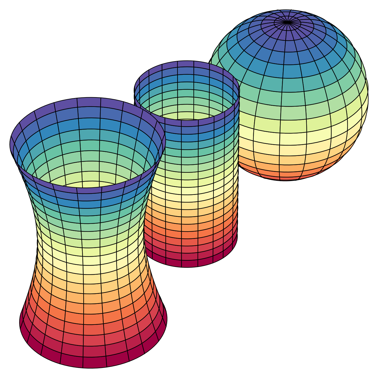
Gaussian Curvature (Wikipedia)

One of the core concepts in Physics is so called metric tensor. This object encodes any kind of geometry. Combined genius of Gauß,  Riemann and their contemporaries lead to such a great idea, probably one of the achievements of human quantitative enlightenment. However, due to notational aspects and lack of obvious pedagogical introduction, making object elusive mathematically. Einstein's notation made this more accessible but still, it requires more explicit explanation.  In this post we disassemble the definition of a distance over any geometry with an alternate notation. 

Disassemble distance over a Riemannian Manifolds

The most general definition of a distance between two infinitesimal points on any geometry, or a fancy word for it, is a Riemannian Manifolds, is defined with the following definitions. Manifold is actually a sub-set of any geometry we are concerned with and Riemannian implies a generalisation.

Definition 1: (Points on a Manifold) Any two points are defined in general coordinates $X$ and $Y$,  They are defined as row and column vectors respectively. In infinitesimal  components. $X = [dx_{1}, dx_{2}, ..., dx_{n}]$ and $Y= [dx_{1}, dx_{2}, ..., dx_{m}]^{T}$. 

Geometric description between two points are defined as tensor product, $\otimes$, that is to say we form a grid, on the geometry. 

Definition 2: (A infinitesimal grid) A grid on a geometry formed by pairing up each point's components, i.e., a tensor product. This would be a matrix $P^{mn}$, (as in points), with the first row $(dx_{1} dx_{1},.....,dx_{1} dx_{n})$ and the last row $(dx_{m} dx_{1},.....,dx_{m} dx_{n})$.

Note that grid here is used as a pedagogical tool, points are actually leaves on the continuous manifold. Now, we want to compute the distance between grid-points, $dS^{n}$, then metric tensor come to a rescue

Definition 3: (Metric tensor) A metric tensor $G^{nm}$ describes a geometry of the manifold that connects the infinitesimal grid to distance, such that $dS^{n}=G^{nm} P^{mn}$.

Note that, these definition can be extended to higher-dimensions, as in coordinates are not 1D anymore. We omit the square-root on the distance, as that''s also a specific to L2 distance.  Here, we can think of $dS^{n}$ a distance vector, and $G^{nm}$ and $P^{mn}$ are the matrices. 

Exercise: Euclidian Metric

A familiar geometry, metric for Euclidian space, reads diagonal elements of all 1 and rest of the elements zero. How the above definitions holds, left as an exercise. 

Conclusion 

We have discuss that a metric tensor, contrary to its name, it isn't a metric per se but an object that describes a geometry, having magic ability to connecting grids to distances. 

Further reading

There are a lot of excellent books out there but a classic Spivak's differential geometry is recommended. 

Mathematical Definition of Heuristic Causal Inference: What differentiates DAGs and do-calculus?

Preamble 

David Hume (Wikipedia)

Experimental design is not a new concept and randomised control trials (RCTs) are our solid gold standard of doing quantitative research, when no apparent physical laws are available to validate observations.  However, it is very expensive to design RCTs, not ethical or either not possible due to logistical reasons in some cases. Then we fall into Causal Inference's heuristic frameworks, such as potential outcomes, matching, and time-series interventions in imagining counterfactuals and interventions. These methods provide immensely successful toolbox for quantitative scientist where by systems do not have any known physical laws. DAGs and do-calculus, differentiates from all these approaches that try to move away from full heuristics. In this post we try to postulate this formally in mathematical terms in the context of causal inference over observational data framework. We established that DAGs and do-calculus bring  mathematically more principled way of practicing causal inference akin to theoretical physics attitude. 

Definition of Heuristic Causal Inference (HeuristicCI) : Observational Data 

Heuristics in general implies an algorithmic approximate solution, usually appear as numerical and statistical algorithms in causal inference whereby full RCT is not available. This can be formalised as follows, 

Definition (HeuristicCI) Given dataset of  $n-$dimensions $\mathscr{D} \in \mathbb{R}^{n}$ observation, having variates of $X=x_{i}$, with each having different sub-sets (categories within $x_{i}$), having at least one category of observations.  We want to test  causal connection between two distinct subsets of $X$,  $\mathscr{S}_{1} , \mathscr{S}_{2}$, given an interventional versions or imagined counterfactual where by at least one of the subset is available,  $\mathscr{S}_{1}^{int} , \mathscr{S}_{2}^{int}$. Using an algorithm $\mathscr{A}$ that processes dataset to test an effect size $\delta$ using a statistic $\beta$,  as follows, $$ \delta= \beta(\mathscr{S}_{1} , \mathscr{S}_{1}^{int})-\beta(\mathscr{S}_{2} , \mathscr{S}_{2}^{int})$$ statistic $\beta$ can be result of a machine learning procedure as well and difference in $\delta$ is only a particular choice, i.e., such as Average Treatment Effect (ATE). The algorithm  $\mathscr{A}$ is called  HeuristicCI.

Many of the non-DAGs and do-calculus methods directly falls into this category, such as potential outcomes, uplift, matching and synthetic controls.  This definition could be quite obvious to practitioners that has a good handle in mathematical definitions. Moreover, HeuristicCI  implies solely data-driven approach to causality inline with Hume's pure-empirical view-point. 

Primary distinction in practicing DAGs that it brings causal ordering naturally [suezen23pco] with scientist's cognitive process encoded, where by HeuristicCI search for statistical effect size that has a causal component in fully data-driven way. However, a HybridCI would entails using DAGs and do-calculus in connection with data driven approaches.

Conclusion

In this short exposition, we introduced HeuristicCI  concept that category of methods that do not use DAGs and do-calculus explicitly in causal inference practice. However, we do not put a well designed RCTs  in this category. Because, as a gold standard approach whereby properly encoded experimental design generates full interventional data reflecting scientist's domain knowledge. 

References and Further reading

• Looper repo : A resource list for causality in statistics, data science and physics
• [suezen23pco] Practical Causal Ordering: Why weighted DAGs are powerful for causal inference?
• Related Wikipedia articles 
• Propensity score matching 
• Synthetic control method
• Difference in Differences
• Uplift Modelling

Please cite as follows:

 @misc{suezen23hci, 

     title = {Mathematical Definition of Heuristic Causal Inference: What differantiates DAGs and do-calculus?}, 

     howpublished = {\url{https://science-memo.blogspot.com/2023/11/heuristic-causal-inference.html}, 

     author = {Mehmet Süzen},

     year = {2023}

}  

Postscript A: Why Pearlian Causal Inference is very significant progress for empirical science? 

Judea Pearl's framework for causality sometimes referred to as “mathematisation of causality”. However, “axiomatic foundations of causal inference” is fair identification, Pearl's contribution to the field is in par with Kolmogorov's axiomatic foundations of probability. Key papers of this axiomatic foundations are published in 1993 (back-doors) [1] and 1995 (do-calculus) [2].  

Original works of Axiomatic foundation for causal inference:

[1] Pearl, J., “Graphical models, causality, and intervention,” Statistical Science, Vol. 8, pp. 266–269, 1993. 

[2] Pearl, J., “Causal diagrams for empirical research,” Biometrika, Vol. 82, Num. 4, pp. 669–710, 1995. 

Resolution of misconception of overfitting: Differentiating learning curves from Occam curves

Preamble 

Occam (Wikipedia)

A misconception that overfitted model can be identified with the  amount of generalisation gap between model's training and test sets over its learning curves is still out there. Even in some prominent online lectures and blog posts, this misconception is now repeated without critical look. In general, this practice unfortunately diffuse into some academic papers and industrial,  practitioners attribute poor generalisation to overfitting. We have provided a resolution of this via a new conceptual identification of complexity plots, so called Occam's curves differentiating from a learning curve. An accessible mathematical definitions here will clarify the resolution of the confusion.   

Learning Curve Setting: Generalisation Gap 

Learning curves explain how a given algorithm's generalisation improves over time or experience, originating from Ebbinghaus's work on human memory.  We use inductive bias to express a model, as model can manifest itself in different forms from differential equations to deep learning.

Definition: Given inductive bias $\mathscr{M}$ formed by $n$ datasets with monotonically increasing sizes  $\mathbb{T} = \{|\mathbb{T}_{0}| > |\mathbb{T}_{1}| > ...> |\mathbb{T}_{n}| \}$. A learning curve $\mathscr{L}$ for $\mathscr{M}$ is expressed by the performance measure of the model over datasets,  $\mathbb{p} = \{ p_{0},  p_{1}, ... p_{n} \}$, hence $\mathscr{L}$ is a curve on the plane of $(\mathbb{T}, p)$.  

By this definition, we deduce that $\mathscr{M}$ learns if $\mathscr{L}$ increases monotonically. 

A generalisation gap is defined as follows. 

Definition: Generalisation gap for inductive bias $\mathscr{M}$ is the difference between its' learning curve $\mathscr{L}$ and the learning curve of the unseen datasets, i.e., so-called training, $\mathscr{L}^{train}$. The difference can be simple difference, or a measure differentiating the gap.

We conjecture the following. 

Conjecture: Generalisation gap can't identify if $\mathscr{M}$ is an overfitted model. Overfitting is about Occam's razor, and requires a pairwise comparison between two inductive biases of different complexities.

As conjecture suggests that generalisation gap is not about overfitting, despite the common misconception. Then, why the misconception? The misconception lies on the confusion of how to produce the curve that we could judge overfitting. 

Occam Curves: Overfitting Gap [Occam's Gap] 

In the case of generating Occam curves, a complexity measure  $\mathscr{C_{i}}$  over different inductive biases $\mathscr{M_{i}}$ plays a role. Then the definition reads. 

Definition: Given $n$ inductive bias $\mathscr{M_{i}}$ formed by $n$ datasets with monotonically increasing sizes  $\mathbb{T} = \{|\mathbb{T}_{0}| > |\mathbb{T}_{1}| > ...> |\mathbb{T}_{n}| \}$. An Occam curve $\mathscr{O}$ for $\mathscr{M}$ is expressed by the performance measure of the model over complexity-dataset size functions  $\mathbb{F} = f_{0}(\{|\mathbb{T}_{0}|, \mathscr{C_{0}}) > f_{1}(|\mathbb{T}_{1}| , \mathscr{C_{1}})> ...> f_{n}(|\mathbb{T}_{n}| , \mathscr{C_{n}}) $; Performance of each inductive bias reads $\mathbb{p} = \{ p_{0},  p_{1}, ... p_{n} \}$, hence Occam curve, $\mathscr{O}$ is a curve on the plane of $(\mathbb{F}, p)$.  

 

Given definition, producing Occam curves are more complicated than simply plotting test and train curves over batches. The ordering in $\mathbb{F}$ forms what is so-called goodness of rank.

Summary and take home

Resolution of misconception of overfitting lies in producing Occam curves to judge the bias-variance tradeoff, not the learning curves of a single model. 

Further reading & notes

• Further posts and a glossary : The concept of overgeneralisation and goodness of rank.
• Double decent phenomenon, it uses Occam's curves, not learning curves.
• We use dataset size as an interpretation of increasing experience, there could be other ways of expressing a gained experience, but we take the most obvious evidence.

Please cite as follows:

 @misc{suezen23rmo, 

     title = {Resolution of misconception of overfitting: Differentiating learning curves from Occam curves}, 

     howpublished = {\url{https://science-memo.blogspot.com/2023/04/Occam-curves.html}}, 

     author = {Mehmet Süzen},

     year = {2023}

}  

Postscript notes

Take home messages

Understanding Generalisation Gap and Occam’s gap

Model selection and evaluations are usually confused by novice and as well as experienced data scientists and professionals doing modelling. There are a lot of misconceptions in the literature, but in practice primary take home messages can be summarised as follows:

1. What is a model? A model is an “inductive bias” of the modeller, a selected parametrised functions for example, a neural network architecture choice. Contrary to many, specific parametrisation of a model (deep learning architecture) is not a different model.
2. A model’s test and training performance difference is about generalisation gap. Overfitting and under-fitting is not about generalisation gap.
3. Overfitting or under-fitting is a comparison problem: How a model deviates from a reference model? This is called Occam’s gap or so called model selection error.
4. Occam’s gap generalises Empirical Risk minimisation over a learning curve.  Empirical risk minimisation itself is not about learning.

How and when a model generalises well and generalisation of empirical risk minimisation are currently an open research topics.

Loschimidt's Paradox and Causality: Can we establish Pearlian expression for Boltzmann's H-theorem?

Boltzmann (Wikipedia)

Preamble

Probably the most important achievement for humans is the ability to produce scientific discoveries, that  helps us objectively understand how nature works and build artificial tools where no other species can.  Entropy is an elusive concept and one of the crown achievements of human race. We question here if causal inference and Loschmidt's paradox can be reconciled. 

Mimicking analogies are not physical

Before even try to understand what is a physical entropy, we should make sure that there is only one kind of physical entropy from thermodynamics, formulated by Gibbs-Boltzmann ($S_{G}$ and $S_{B}$).  Other entropies such as Shannon's information entropy are all analogies to physics, and mimicking concepts.

Why counting microstates are associated with time?

The following definition of entropy is due to Boltzmann but Gibbs' formulation tend to provide equivalence, technically different formulations aside, they are actually equivalent.

Definition 1: An entropy of a macroscopic material is associated with larger number of states its constituted elements take different states, $\Omega$. This is associated with $S_{B}$, Boltzmann's entropy.  

Now, as we know from basic thermodynamics classes that entropy change of a system can not decrease, so the time's arrow. 

Definition 2: Time's arrow is identified with change in entropy of material systems, that $\delta S \ge 0$.

We put aside the distinction between open and close systems and equilibrium and non-equilibrium dynamics, but concentrate on how come counting system's state's are associated with time's arrow? 

Loschimidt's Paradox: Irreversible occupancy on discrete states and causal inference

The core idea probably can be explained via discrete lattice and occupancy on them over chain of dynamics. 

Conjecture 1: Occupancy of $N$ items on $M$ discrete states, $M>N$, evolving with dynamical rules $\mathscr{D}$ necessarily increases $\Omega$, compare to the number of sampling if it were $M=N$. 

This conjecture might explain the entropy increase, but irreversibility of the dynamical rule $\mathscr{D}$ is required addressing Loschimidt's Paradox, i.e., how to generate irreversible evolution given time-reversal dynamics. Actually, do-calculus may provide a language to resolve this, by inducing interventional notation on Boltzmann's H-theorem with Pearlian view. The full definition of H-function is a bit more involved, but here we summarise it in condensed form with a do operator version of it.

Conjecture 2 (H-Theorem do-conjecture): Boltzmann's H-function provides a basis for entropy increase, it is associated with conditional probability of a system $\mathscr{S}$ being in state $X$ on ensemble $\mathscr{E}$. Hence, $P(X|\mathscr{E})$. Then, an irreversible evolution from time-reversal dynamics should use interventional notation, $P(X|do(\mathscr{E}))$. Then information on how time reversal dynamics leads to time's arrow encoded on, how dynamics provides an interventional ensembles, $do(\mathscr{E})$.

Conclusion

We provided some hints on why would counting states lead to time's arrow, an irreversible dynamics.  In the light of the development of mathematical language for causal inference in statistics, the concepts are converging. Along with understanding Loschmidt's Paradox via do-calculus, it can establish an asymmetric notation. Loschmidt's question is long standing problem in physics and philosophy with great practical implications in different physical sciences.

Further reading

• Loschimid's Paradox
• H-Theorem
• do-Calculus revisited, J. Pearl (2012) pdf
• Causal Inference : Looper Repository for collection of resources.
• H-theorem do-conjecture, M. Süzen,  arxiv:2310.01458 (2023) 

Please cite as follows:

 @misc{suezen23lpc, 

     title = {Loschimidt's Paradox and Causality: Can we establish Pearlian expression for Bolztmann's H-theorem?}, 

     howpublished = {\url{https://science-memo.blogspot.com/2023/02/loschimidts-do-calculus.html}}, 

     author = {Mehmet Süzen},

     year = {2023}

}  

@article{suzen23htd,

    title={H-theorem do-conjecture},

    author={Mehmet Süzen},

    preprint={arXiv:2310.01458},

    url = {https://arxiv.org/abs/2310.01458}

    year={2023}

}